2025-02-25發表2025-02-25更新9 分鐘讀完 (大約1327個字)

將資料可視化，Python Pandas 及 Matplotlib 簡介

Pandas

根據 Pandas 官方網站介紹，Pandas 專門處理所謂的 Tabluar Data，也就是像是 Excel、資料庫的表格型資料，在 Pandas 中儲裡 Tablular 的基本資料格式稱作 Data Frame（也簡稱 DF）。

官網的 DataFrame 圖片

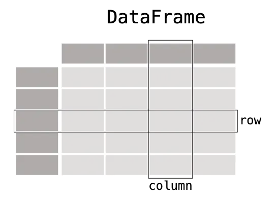
Pands 支援各種不同格式的讀寫，將讀取的資料轉成 DF 或是再轉成各種格式，包含基礎的 CSV, XLS, JSON，還有更多如 HTML, SQL 等等。

基礎操作

假設現在有一組 Time Series Data，由一個 Array 組成，每個元素有 Time 及 Speed，我們將這組資料丟入 Pandas Data Frame 中處理，就能做一些基本的統計。

像是計算速度的算術平均、最小最大值、中位數、標準差等等。

import pandas as pd

data = [
    {"time": 1, "speed": 1},
    {"time": 2, "speed": 2},
    {"time": 3, "speed": 3},
    {"time": 4, "speed": 5},
    {"time": 5, "speed": 8},
    {"time": 6, "speed": 10},
    {"time": 7, "speed": 11},
    {"time": 8, "speed": 11},
]

df = pd.DataFrame(data)

print("DataFrame Header:")
print(df.head())
print("\nSpeed Statistics:")
print(f"Average Speed: {df['speed'].mean()}")
print(f"Min Speed: {df['speed'].min()}")
print(f"Max Speed: {df['speed'].max()}")
print(f"Median Speed: {df['speed'].median()}")
print(f"Standard Deviation: {df['speed'].std()}")

以下為實際輸出的內容

DataFrame Header:
   time  speed
0     1      1
1     2      2
2     3      3
3     4      5
4     5      8

Speed Statistics:
Average Speed: 6.375
Min Speed: 1
Max Speed: 11
Median Speed: 6.5
Standard Deviation: 4.138236339311712

除了基本的統計操作之外，也能做資料的篩選、轉換。

例如以下的程式碼，將速度大於等於 10 的資料篩選保留下來；將速度的數值轉換成其他單位。

# Filtering
speeding_df = df[df["speed"] >= 10]
print(f"Speeding data:\n{speeding_df}")

# Conversion
kmh_speed_df = df.copy()
kmh_speed_df["speed"] = kmh_speed_df["speed"] * 3.6  # Convert m/s to km/h
print(f"\nSpeeds in km/h:\n{kmh_speed_df}")

除此之外，也能和繪圖的 Library 整合，用圖表的方式呈現，讓我們來看看與 Matplotlib 共同使用的方式。

Matplotlib

將剛剛的 Data Frame 搭配 Matplotlib，簡單呼叫 .plot() 和 .show() 即可繪製出圖形

import matplotlib.pyplot as plt

df["speed"].plot()
plt.show()

以下為輸出的圖形：

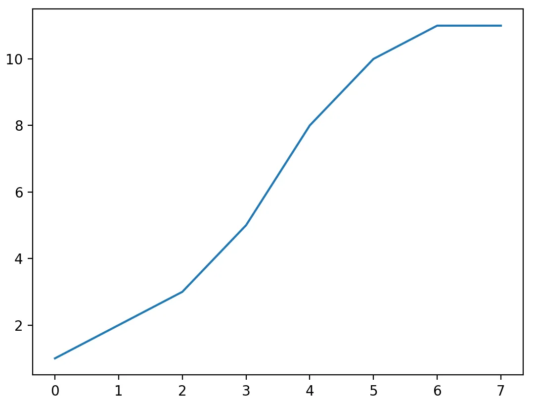
預設的 x 軸為 Array 的 Index，而 Y 軸則是我們所指定的 speed 欄位。

Matplotlib 簡介及基礎操作

Matplotlib 是 Python 常見的繪圖 Library，其命名來源為 MATLAB, plot, and library 所組成的，其中的 MATLAB 全稱為 Matrix Laboratory（矩陣實驗室），是一種用於演算法開發、資料視覺化的軟體。而 Matplotlib 就是在 Python 上提供類似 MATLAB 繪圖介面的函式庫。

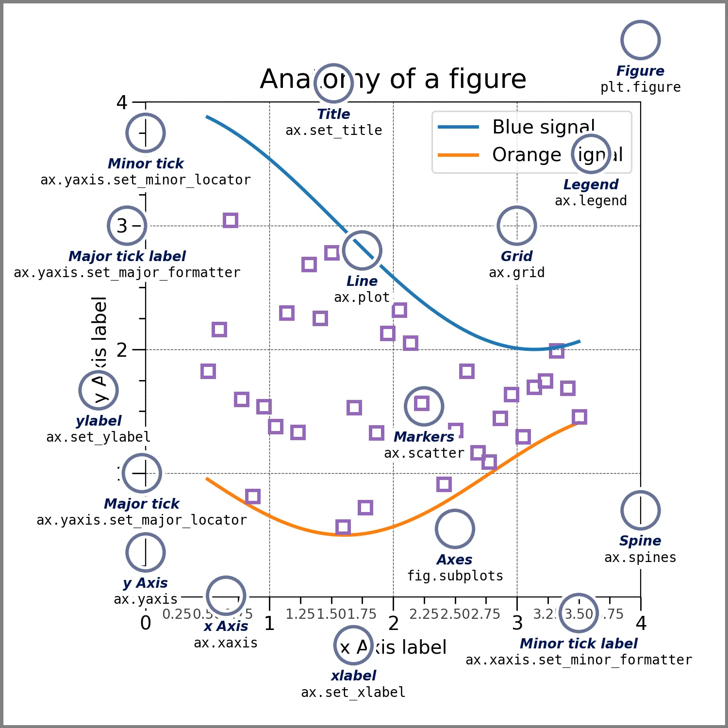
Matplotlib 會將資料繪製在 Figure 上，而所謂的 Figure 可以想像成一張畫布，畫布上有一到多個 Axes，每個 Axes 有自己的坐標系。

而 Figure 上還可以透過 Artist 畫出不同的元素，例如 Text、Line 等等。像是下圖的 Figure，裡面的顯示的內容如 plot, title, xlabel, ylabel 都屬於 Artist 繪製出來的。

官方的 Figure 解說圖

有了基礎的概念，我們可以沿用上個小節使用的 Pandas Data Frame，來更詳細的繪製出時間-速度圖。

時間-速度圖

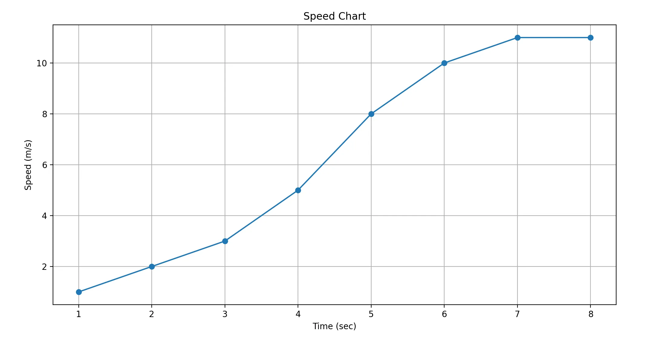
import matplotlib.pyplot as plt

plt.figure(figsize=(12, 6))
plt.plot(df["time"], df["speed"], marker="o")
plt.title("Speed Chart")
plt.xlabel("Time (sec)")
plt.ylabel("Speed (m/s)")
plt.grid(True)
plt.show()

我們在此 Figure 中加上了 title, label 和 grid 等 Artist 的元素。

Matplotlib 之 Subplots

我們已經能繪製時間-速度圖了，但如果我們想加上一些其他的元素，例如我們有一台車的速度及狀態資訊，當車輛在速度變快時，實際上是在踩油門（Accelerating, acc），而煞車時（Decelerating, dec）能看到加速度變小，能否將速度和踩油門煞車同時放在表上呢？

前面提到一個 Figure 可以有一到多個 Axes 對吧，要達成同一個 Figure 上顯示多張圖表，我們可以透過 Subplots 做到。

import pandas as pd

data = [
    {"time": 1, "speed": 1, "state": "acc"},
    {"time": 2, "speed": 2, "state": "acc"},
    {"time": 3, "speed": 3, "state": "acc"},
    {"time": 4, "speed": 5, "state": "acc"},
    {"time": 5, "speed": 8, "state": "acc"},
    {"time": 6, "speed": 10, "state": "dec"},
    {"time": 7, "speed": 11, "state": "dec"},
    {"time": 8, "speed": 11, "state": "mov"},
]

df = pd.DataFrame(data)

我們先將原本的 data 加上一個欄位 state，裡面有不同列舉（Enum）：acc, dec, mov，分別對應到加速、減速和正常移動的狀態。當加減速時，可以期望實際的速度增加或減少的速度改變的比較快。

有了這樣的資料，就可以來試試使用 Subplots 來畫圖

import matplotlib.pyplot as plt

fig, (ax1, ax2) = plt.subplots(2, 1, figsize=(12, 8), sharex=True)

ax1.plot(df["time"], df["speed"], marker="o")
ax1.set_ylabel("Speed (m/s)")
ax1.grid(True)

ax2.plot(df["time"], df["state"], marker="o")
ax2.set_ylabel("State")
ax2.grid(True)

ax2.set_xlabel("Time (sec)")

plt.tight_layout()
plt.show()

呼叫 plt.subplots 時傳入我們要建立幾個 Axes，並且指定共用 x 軸（sharex=True），就能畫出下圖這樣，共用 x 軸疊在一起的圖形。

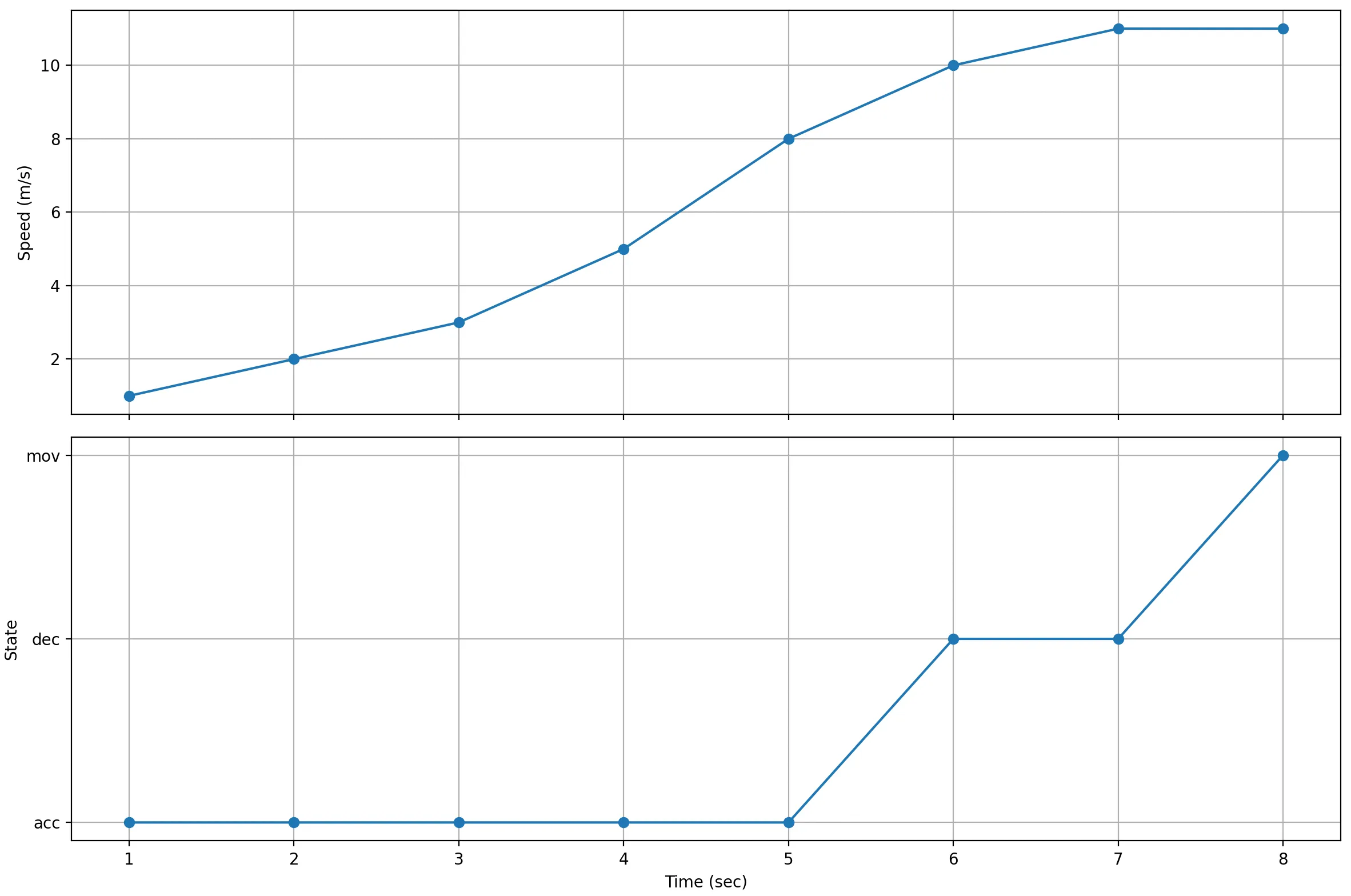
如此一來便能對比不同狀態（加減速）時，速度的變化是否真的符合我們的預期了！

參考資料

#python